Mass-Spring-Damper System

Lesson Scope

This lesson supplements an undergraduate course in differential equations by using the mass-spring-damper (MSD) model to connect second-order linear ODEs to engineering vibration problems.

You will:

connect common engineering examples to the MSD model,
derive the governing equation from a free-body diagram,
analyze the unforced response and interpret the three damping regimes (underdamped, critically damped, and overdamped), and
study the forced response, including resonance, beats, and how damping changes steady-state amplitude and phase.

Throughout, interactive figures and “Quick Checks” are used to help you build intuition and check understanding. Hover-to-define terms provide concise definitions inline, and “Show Work” sections are available for readers who want more derivation detail.

Background

The mass-spring-damper (MSD) system is a simplified mathematical model of many real-world systems. Figure 1 shows the basic system considered. The objective is to find the motion of the mass as a function of time. The mass is connected to the wall via a spring which provides a restoring force when stretched and a resisting force when compressed. This motion is opposed by a damper, which is represented by wall friction in Figure 1.

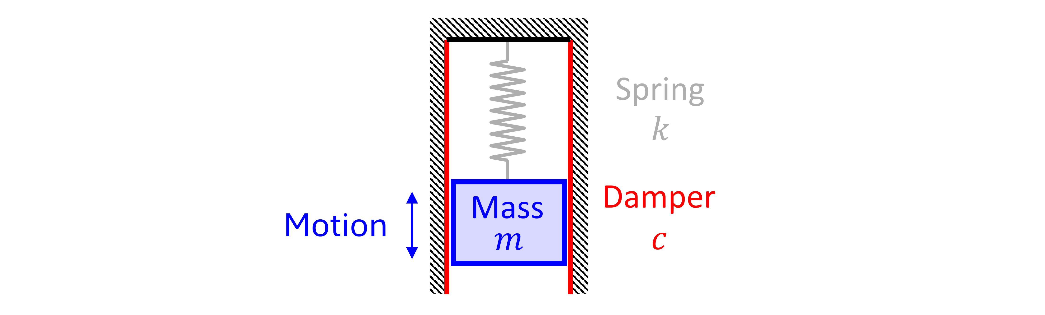
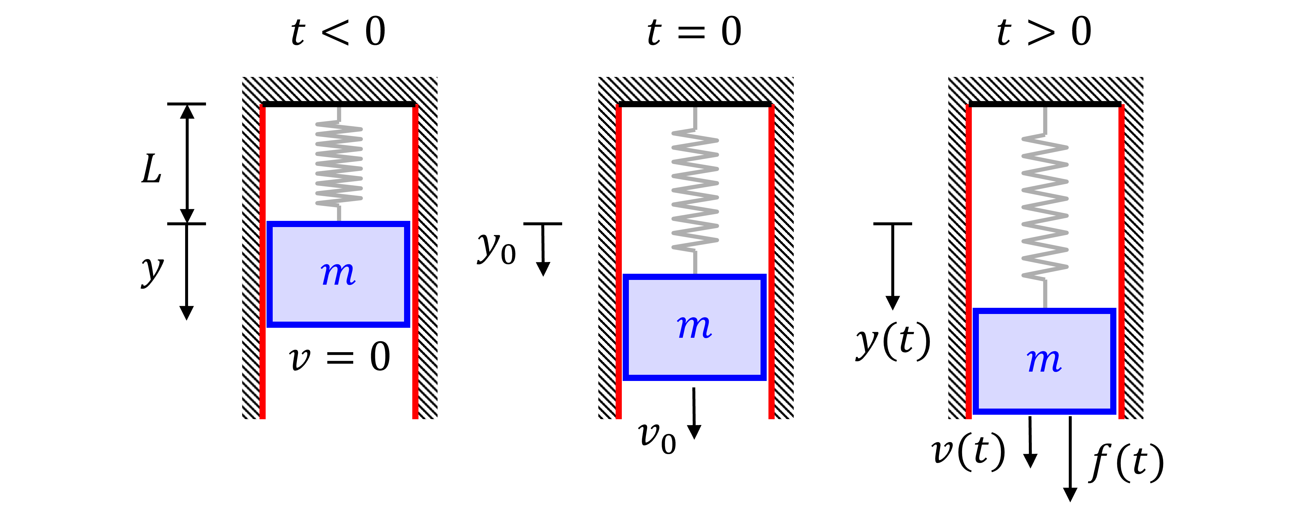
Figure 2 shows the MSD system at three different states: when the mass is at rest t<0, the motion’s initial conditions t=0, and once motion begins t>0.
When the mass is at rest (in an equilibrium state), the spring is stretched by length L. It’s convenient to define our coordinate system, y, based on position of the mass at its rest state so that displacement represents the distance from equilibrium.
At t=0, the mass is displaced by a distance y_0 with velocity v_0. This causes the mass to move for t > 0. Once in motion, we can have either an unforced system or a forced system with the external force f(t).

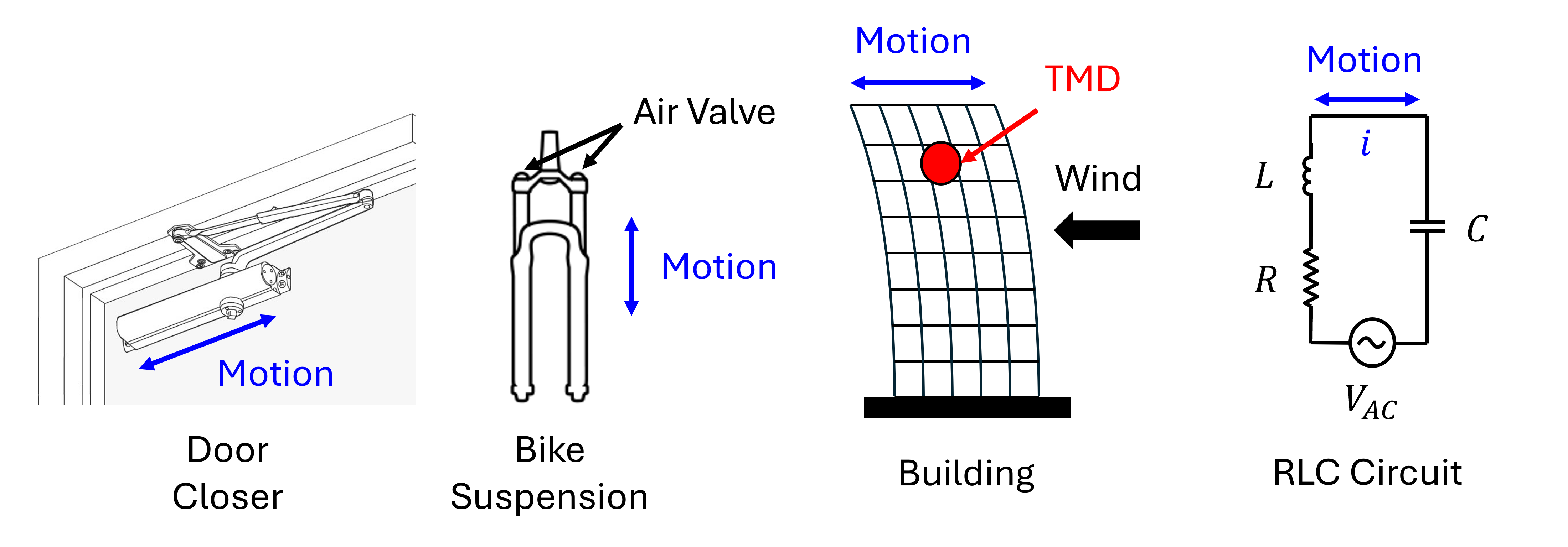
To gain an understanding of the real-world applications, we’ll now consider four examples of MSD systems (shown in Figure 3 along with a table summary Table 1):

Door closer - Opening the door loads a spring in the door closer mechanism, storing energy; when released, the spring drives the door shut while a hydraulic piston forces oil through a small orifice, providing damping that prevents the door from slamming.
Bike front suspension - A bump compresses the fork, increasing pressure in the air chamber (spring) that stores energy and pushes the fork back out, while a hydraulic damper controls oil flow to limit how quickly the fork compresses and rebounds so the bike doesn’t bounce.
Building - A building sways like a mass-spring-damper in wind or earthquakes, with the structure’s mass moving against the stiffness of columns/walls (spring) and energy lost through material/structural damping (damper). In extreme cases the wind forcing frequency can achieve resonance with the building’s natural frequency, which can have catastrophic consequences. Some very tall buildings counter this with a tuned mass damper (TMD).
RLC circuit - An RLC circuit is the electrical analog of a mass-spring-damper, where inductance acts like mass (inertia), capacitance like a spring (stored energy), and resistance like damping (energy dissipation).

Table 1: MSD real-world examples and their physical analogies

Example	Motion	Mass	Spring	Damper	Force
Door Closer	piston moving	door	internal spring	hydraulic damping	pushing door
Bike Suspension	vertical motion of bike	bike frame	coil/air spring	hydraulic damper (oil)	bumpy ground
Building	sway	building	stiffness	structural damping	wind
RLC Circuit	current	inductance	elastance (1/C)	resistor	applied voltage

Governing Equation

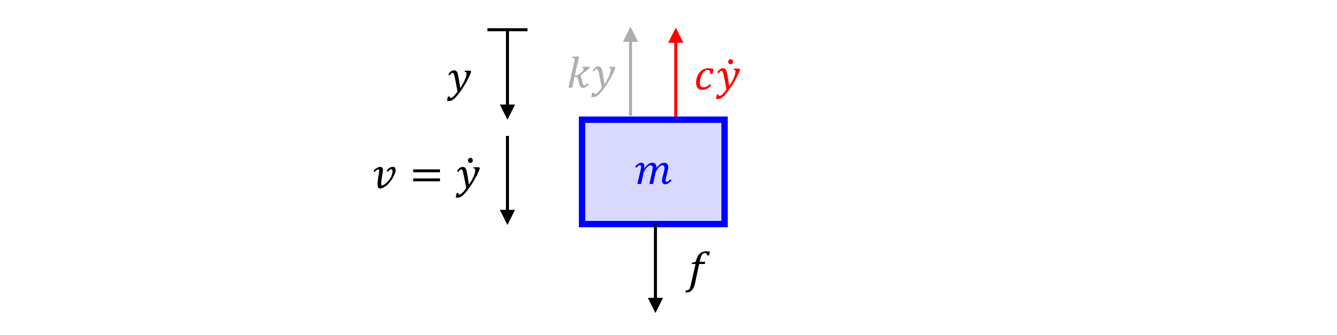
To derive the governing equation for the mass’s motion, we first write a force balance via a free body diagram. Figure 4 shows the forces acting on the mass. For positive displacement, y>0, the spring is stretched and gives a force in the negative y direction. For negative displacement, the spring is compressed and gives a force in the positive y direction. In both cases the spring force opposes the displacement, which may be written as F_s = -ky where k is the spring constant. Similarly, the damper opposes the velocity of the mass. This is just like surface friction opposing the motion of a block sliding or drag slowing a ball thrown through the air. This gives the force F_d = -c \dot{y}, where an overhead dot denotes a derivative with respect to time. The linear relationship between force and velocity is an approximation, but accurate for most applications. Finally the external force, f(t), is defined to be positive in the positive y direction.

Next we apply Newton’s second law of motion \begin{aligned} \sum F_y &= m a = m \ddot{y} \\ &= f(t) - k y - c \dot{y} \end{aligned}

Rewriting gives the final governing equation m \ddot{y} + c \dot{y} + k y = f(t) \tag{1} This equation is a second-order, linear, nonhomogeneous ordinary differential equation (ODE) with constant coefficients. Let’s define each of these terms.

The order of an ODE is the highest order derivative in the equation. In this case \ddot{y} is the highest order derivative, so the ODE is second order.

An ODE is linear if y and its derivatives appear only to the first power and are not multiplied together; coefficients may depend on the independent variable. For example, a(t)\dot{y} is linear but y\dot{y} is nonlinear. A principal feature of linear ODEs is solutions can be superposed.

A homogeneous ODE is linear but with no external forcing term. The external force, f(t), in Equation 1 makes the equation nonhomogeneous. This distinction has important implications in solution strategies.

An ordinary differential equation only has derivatives with respect to one independent variable; as opposed to a partial differential equation which has derivatives with respect to two or more independent variables.

Each of these classifications has a significant influence on solution properties and strategies. Next we’ll discuss the unforced system, f(t) = 0.

The Unforced System

In the unforced system, the motion is driven only by the initial displacement and velocity (no external force). This section shows how the solution depends on damping and how to interpret the resulting time response.

Analytical Solution

In the unforced system we set f = 0 in Equation 1 and get m \ddot{y} + c \dot{y} + k y = 0 \tag{2}

This equation is now homogeneous, allowing us to apply the superposition principle to obtain the general solution.

In general, homogeneous ODEs with constant coefficients admit exponential solutions, i.e. solutions of the form y(t) = a e^{\lambda t} where \lambda is the growth/decay rate and can be complex. For example, the first-order ODE \dot{y}+by=0 yields exponential decay y = a e^{-bt} for b>0.

This suggests we should try to solve Equation 2 assuming y = a e^{\lambda t}. Substituting in Equation 2 yields a m \lambda^2 e^{\lambda t} + a c \lambda e^{\lambda t} + a k e^{\lambda t} = (m \lambda^2 + c \lambda + k)a e^{\lambda t} = 0 which is reduced to m \lambda^2 + c \lambda + k = 0. \tag{3} Equation 3 is known as the characteristic equation. This can be solved using the quadratic formula \lambda_{1,2} = \frac{1}{2m}\left( -c \pm \sqrt{c^2 - 4 m k} \right) \tag{4} where the subscript 1, 2 represents the fact there are two solutions to the characteristic equation corresponding to the “+” or “-” sign.

We’ve now solved the equation! We assumed y = a e^{\lambda t} and found \lambda must be Equation 4 by solving the characteristic equation. Using the superposition principle, the general solution is then y = a_1 e^{\lambda_1 t} + a_2 e^{\lambda_2 t} \tag{5} The value of the constants a_1 and a_2 can be determined by the initial conditions, y(0)=y_0 and \dot{y}(0) = v_0. Since the ODE is second-order, we need two initial conditions.

Note in Equation 4 that if c^2 < 4mk then \lambda is complex! This has important implications on the solution behavior and will be discussed next.

Undamped

First let’s consider the undamped case by setting c=0. Then Equation 4 becomes \lambda_{1,2} = \pm \sqrt{\frac{k}{m}} i = \pm \omega_n i \tag{6} where i \equiv \sqrt{-1} is the imaginary number and \omega_n is known as the natural frequency of the system.

What happens when \lambda is imaginary? Recall Euler’s formula e^{ix} = \cos x + i \sin x. Substituting Equation 6 into Equation 5 and applying Euler’s formula yields

Show Work

\begin{align*} y &= a_1 e^{i\omega_n t} + a_2 e^{-i\omega_n t} \\ &= a_1 \left( \cos{\omega_n t} + i \sin{\omega_n t} \right) + a_2 \left( \cos{\omega_n t} - i \sin{\omega_n t} \right) \\ &= b_1 \cos{\omega_n t} + b_2 \sin{\omega_n t} \end{align*} where the definitions b_1 \equiv a_1 + a_2 and b_2 \equiv (a_1 - a_2) i are made.

In order for b_1 and b_2 to be real numbers, a_1 and a_2 must be complex conjugates of each other, a_2 = \overline{a_1}.

The choice of variable names is arbitrary so we return to using a_1 and a_2 in the final equation.

y = a_1 \cos{\omega_n t} + a_2 \sin{\omega_n t} \tag{7} Once again we can solve for a_1 and a_2 given the initial conditions. This gives the final solution. y = y_0 \cos{\omega_n t} + \frac{v_0}{\omega_n} \sin{\omega_n t} \tag{8}

Now let’s explore the behavior of this solution via the interactive figure below.

Through this demo we’ve shown that the undamped solution is sinusoidal with frequency \omega_n which is inherent to the system’s properties (mass and spring constant) and NOT the initial conditions.

An undamped system is unrealistic, however. There is always some source of friction or dissipation which decays motion. Next we’ll show how damping affects solution behavior.

Damped

Recall the solution, \lambda_{1,2}, to the characteristic equation, Equation 4. We had hinted that the behavior of the solution depends on the magnitude of c^2 versus 4mk. In other words, the strength of the damping plays a critical role in the behavior of the MSD system.

The analysis is simplified if we introduce a new parameter \zeta defined to be \zeta \equiv \frac{c}{2m\omega_n} where \omega_n \equiv \sqrt{k/m} is the natural frequency from the undamped case. Using these definitions simplifies the characteristic roots: \lambda_{1,2} = \omega_n \left( -\zeta \pm \sqrt{\zeta^2 - 1} \right). Now it’s clear that the solution behavior (real or complex) only depends on the parameter \zeta. Note \zeta is essentially a non-dimensional damping coefficient.

Let’s see how the solution changes now that we’ve introduced this new parameter.

Now that we qualitatively understand the different behavior between under, over, and critically damped systems, let’s look into the specifics of each.

Underdamped

For \zeta < 1 the system is underdamped and the solution is oscillatory with an exponentially decaying amplitude. The solution for the underdamped system is

Show Work

For \zeta < 1, \lambda_{1,2} = -\omega_n \zeta \pm \omega_d i where \omega_d \equiv \omega_n \sqrt{1- \zeta^2}. The characteristic roots are complex.

Substitute \lambda into the unforced solution and we get \begin{align*} y &= a_1 e^{(-\omega_n \zeta + i \omega_d) t} + a_2 e^{(-\omega_n \zeta - i \omega_d) t} \\ &= e^{(-\omega_n \zeta)t} \left( a_1 e^{i \omega_d t} + a_2 e^{-i \omega_d t} \right) \\ &= e^{(-\omega_n \zeta)t} \left( a_1' \cos{\omega_d t} + a_2' \sin{\omega_d t} \right) \end{align*} where in the last step Euler’s formula was used and prime denotes new constants, similar to what was done for the undamped case.

y = e^{-\omega_n \zeta t} \left( a_1 \cos \omega_d t + a_2 \sin \omega_d t \right) \tag{9} where \omega_d = \omega_n \sqrt{1-\zeta^2} is the damped oscillation frequency. For low damping, \zeta \ll 1, the damped frequency is the same as the natural frequency. However, as damping increases the damped frequency decreases.

The exponential term e^{-\omega_n \zeta t} causes the oscillation amplitude to decay over time. In the demo we showed that this exponential term forms an envelope over the oscillations, representing the maximum amplitude of the oscillations at any time. We also showed that higher natural frequencies decay faster than lower natural frequencies.

In engineering, underdamping may be desired if quick response is desired (reaching y=0 fastest) and a little overshoot is okay. This is true for robotic arms where quick motion is essential and controllers can respond overshooting. Overdamping, conversely, can result in delayed response times.

Critically Damped

For \zeta = 1 the system is critically damped and the solution is non-oscillatory with fast exponential decay from initial conditions. This has the solution

Show Work

For \zeta = 1, \lambda = -\omega_n \zeta. This corresponds with a double root of the characteristic equation. This means that we no longer have two linearly independent solutions and we have to find a new independent solution. This involves the reduction of order method which is beyond the scope of this lesson. For now, let’s assume it has the form y_2 = a_2 te^{\lambda t}. Then using y_1 = a_1 e^{\lambda t} we get y = y_1 + y_2 = (a_1 + a_2 t)e^{-\omega_n \zeta t}

y = (a_1 + a_2 t) e^{-\omega_n t}.

This solution corresponds with the least amount of time to reach stationary conditions. The solution can cross y=0 at most one time when a_1 + a_2 t = 0.

A critically damped system is desired if you want motion damped quickly without oscillation. This is true for door closers. If underdamped, the door slams shut or oscillates. If overdamped, the door takes too long to close.

Overdamped

For \zeta > 1 the solution is overdamped and is non-oscillatory with slow exponential decay from initial conditions. This has the solution

Show Work

For \zeta > 1, \lambda_{1,2} = -\omega_n \left( \zeta \pm \sqrt{\zeta^2-1} \right) corresponding to two real characteristic roots. Substituting into the general solution gives y = a_1 e^{-\omega_n t \left( \zeta + \sqrt{\zeta^2-1}\right)} + a_2 e^{-\omega_n t \left( \zeta - \sqrt{\zeta^2-1} \right)}

y = a_1 e^{-\omega_n t \left( \zeta + \sqrt{\zeta^2-1}\right)} + a_2 e^{-\omega_n t \left( \zeta - \sqrt{\zeta^2-1} \right)}

This has two decay rates: one fast and one slow with the slow rate dominating over long times and both interacting for short times.

In some cases, overdamping is desired. Industrial shock absorbers (end-of-stroke dampers) are commonly selected or adjusted so the overall response is near-critically damped or slightly overdamped, bringing a moving load to rest without oscillation or rebound. An underdamped (oscillatory) response can cause repeated impacts that damage nearby components or fixtures, so minimizing bounce is often the safer design choice.

Next we’ll discuss the forced system, when f(t) \neq 0.

The Forced System

In the forced system, an external input f(t) continually injects energy into the system. This section focuses on periodic forcing, where the relationship between forcing frequency and the system’s natural frequency leads to resonance, beats, and a steady-state response with a well-defined amplitude and phase.

Undamped

Previously we’ve only dealt with homogeneous ODEs. Now we have a nonhomogeneous ODE when f(t) \neq 0. For linear nonhomogeneous ODEs we can get the general solution by adding a particular solution to the homogeneous solution. That is y(t) = y_h(t) + y_p(t) \tag{10} where y_h = a_1 y_1 + a_2 y_2 is the homogeneous solution to Equation 2 with arbitrary constants, a_1 and a_2, (discussed previously in the unforced section) and y_p is a particular solution to Equation 1 with no arbitrary constants.

General methods for finding the particular solution are difficult and beyond the scope of this lesson. Instead we’ll only consider forcing of the form f(t) = f_0 \cos \omega_f t. which has many real-world implications. We’ve now introduced a new important parameter, \omega_f, the forcing frequency. The forcing frequency interacts with the natural frequency of the system in interesting ways.

To understand this interaction between the forcing and natural frequency, let’s first consider the undamped system (c=0) with periodic forcing and its solution. The governing equation is m \ddot{y} + k y = f_0 \cos \omega_f t \tag{11} and the corresponding homogeneous solution was found previously, Equation 7. The particular solution is found using the method of undetermined coefficients. This method can only be applied if the force, f(t), has specific functional forms. If it meets this criterion, then the particular solution will be a known functional form with undetermined coefficients. For a sine or cosine function with frequency \omega_f, the particular solution is y_p = b_1 \cos{\omega_f t} + b_2 \sin{\omega_f t}. \tag{12} The undetermined coefficients, b_1 and b_2, are found by substituting the particular solution into Equation 11. This leads to a system of equations for the coefficients which is solved to yield b_1 = \frac{f_0}{m\left( \omega_n^2 - \omega_f^2 \right)}, \quad b_2 = 0. Then we superpose the homogeneous and particular solutions to get the general solution y(t) = a_1 \cos{\omega_n t} + a_2 \sin{\omega_n t} + \frac{f_0}{m\left( \omega_n^2 - \omega_f^2 \right)} \cos{\omega_f t} \tag{13} where a_1 = y_0 - \frac{f_0}{m\left( \omega_n^2 - \omega_f^2 \right)}, \quad a_2 = \frac{v_0}{\omega_n} were found using the initial conditions. Note the coefficients go to infinity when \omega_f = \omega_n. In this situation we must assume a different form for the particular solution because y_p, Equation 12, is not linearly independent from y_h, Equation 7, when \omega_f = \omega_n. Instead we must choose a trial function y_p = b_1 t \cos{\omega_f t} + b_2 t \sin{\omega_f t}. Then we can repeat the process and get the general solution when the forcing and natural frequencies match: y(t) = a_1 \cos{\omega_n t} + a_2 \sin{\omega_n t} + \frac{f_0}{2m\omega_n} t \sin{\omega_n t}. \tag{14}

Below is a demo to explore the behavior of the undamped solution. The solid line corresponds with the undamped solution (Equation 13 and Equation 14) and the dashed line corresponds with the envelope of this solution.

This demo demonstrated the concepts of resonance and beats.

Resonance occurs when the forcing frequency matches the natural frequency of the system. This results in amplification of the motion over time. This is similar to swinging. To increase your height, you propel yourself forward at the same time the swing starts to move forward. In other words, your forcing frequency is aligned with the swinging frequency. Resonance is also why singing at the right pitch (forcing frequency) can cause a glass (natural frequency) to break. In some cases resonance can be catastrophic. For tall buildings (or other large civil structures), wind can generate a forcing frequency which resonates with the building, capable of causing damage if oscillation amplitudes are large enough. In engines or other periodic forcing machines it’s important to make sure none of the other components have the same natural frequency as the forcing, otherwise vibrations could be amplified.

Beats occur when the forcing frequency is close to the natural frequency. Because the forcing frequency and natural frequency of the system are slightly different, forces slowly go from in phase (amplification) to out of phase (cancellation), generating low frequency beats. Guitar tuning utilizes this feature. When you tune a guitar, you listen for beats (slow pulsing) that happens when the string and a reference note are slightly different in frequency. As you tune closer, the beat rate slows, and when the beats nearly disappear the pitches match.

Damped

Zero damping is unrealistic. Real systems have some amount of damping. In this section we’ll introduce damping to the forced system and how it affects resonance.

With damping we will be solving m \ddot{y} + c\dot{y} + k y = f_0 \cos(\omega_f t) \tag{15} and again the solution has homogeneous and particular parts. The particular solution is the same as the undamped case, Equation 12. For the transient (homogeneous) part we focus on the common lightly damped case \zeta < 1, so the homogeneous solution matches the unforced underdamped form in Equation 9.

We repeat the process as was done in the undamped case and get the general solution y(t) = y_h(t) + y_p(t) where y_h = e^{-\omega_n \zeta t} \left( a_1 \cos \omega_d t + a_2 \sin \omega_d t \right), with a_1 and a_2 determined from initial conditions and y_p = b_1 \cos{\omega_f t} + b_2 \sin{\omega_f t} with the coefficients b_1 = \frac{(f_0/k)(1-r^2)}{(1-r^2)^2 + (2\zeta r)^2}, \quad b_2 = \frac{(f_0/k)(2\zeta r)}{(1-r^2)^2 + (2\zeta r)^2} and r=\omega_f/\omega_n is the frequency ratio.

Note now y_h decays to zero as t\to \infty as opposed to the undamped case where y_h is an undecaying sinusoid. This means that for long times (roughly after t \gtrsim 3/(\zeta \omega_n)) after the initial motion the particular solution will dominate. Therefore, when considering damped resonance it is useful to only consider the particular solution and its maximum amplitude. This is often called practical resonance.

We can understand practical resonance by rewriting the particular solution (using trigonometric identities) as y_p = A \cos (\omega_f t - \phi) where A is the amplitude of y_p and \phi is the phase angle or phase lag because it measures the lag of the output behind the input. These are evaluated as A = \sqrt{b_1^2 + b_2^2} = \frac{f_0/k}{\sqrt{(1-r^2)^2 + (2\zeta r)^2}}, \quad \tan \phi = \frac{b_2}{b_1} = \frac{2\zeta r}{1-r^2}.

Let’s now see how the response amplitude and phase are influenced by damping and forcing frequency via an interactive demo. The figure on the left plots amplitude versus the frequency ratio \omega_f/\omega_n. The response amplitude is normalized by the steady forcing displacement (f_0/k) and so a value greater than one corresponds with amplification relative to the input.