Separation Modeling
This page briefly describes preliminary research on smooth body separation, specifically for flow over the prolate spheroid.
Background
The objective of this work is to predict the “separation location” for flow over a prolate spheroid. Figure 1 provides a schematic picture of this flow. Flow hits the spheroid with some angle of attack (AOA) or drift angle, \beta.
Then a viscous layer forms on surface called a boundary layer. The adverse pressure gradient slows the boundary layer until the momentum of the fluid isn’t enough to remain attached. The flow separates and a pair of counter-rotating vortices are generated at the separation location. These vortices advect downstream, forming a vortex sheet as new vortices are generated.
This vortex sheet is called the wake and it plays a huge role in the forces felt on the body. And the separation location, being the starting point of wake development, plays a critical role in force and moment predicts on bodies like this. The separation location is a function of the axial coordinate, X, and the azimuthal angle, \phi.
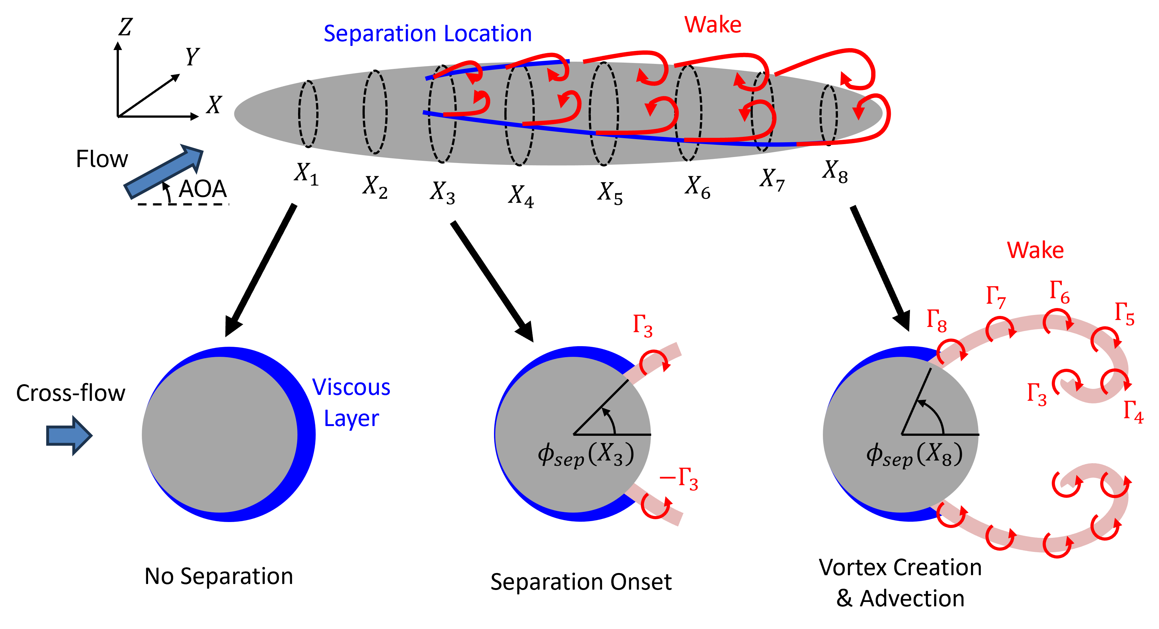
Figure Figure 2 shows “closed” versus “open” separation. Closed separation has a continuous separation curve and forms a wake similar to a separation bubble. Open separation, conversely, does not have a continuously connected separation curve and two vortex sheets, as described previously. Flow over spheroid can have either closed or open separation depending on the AOA or drift angle. Low drift angles have closed separation whereas high drift angles have open separation.
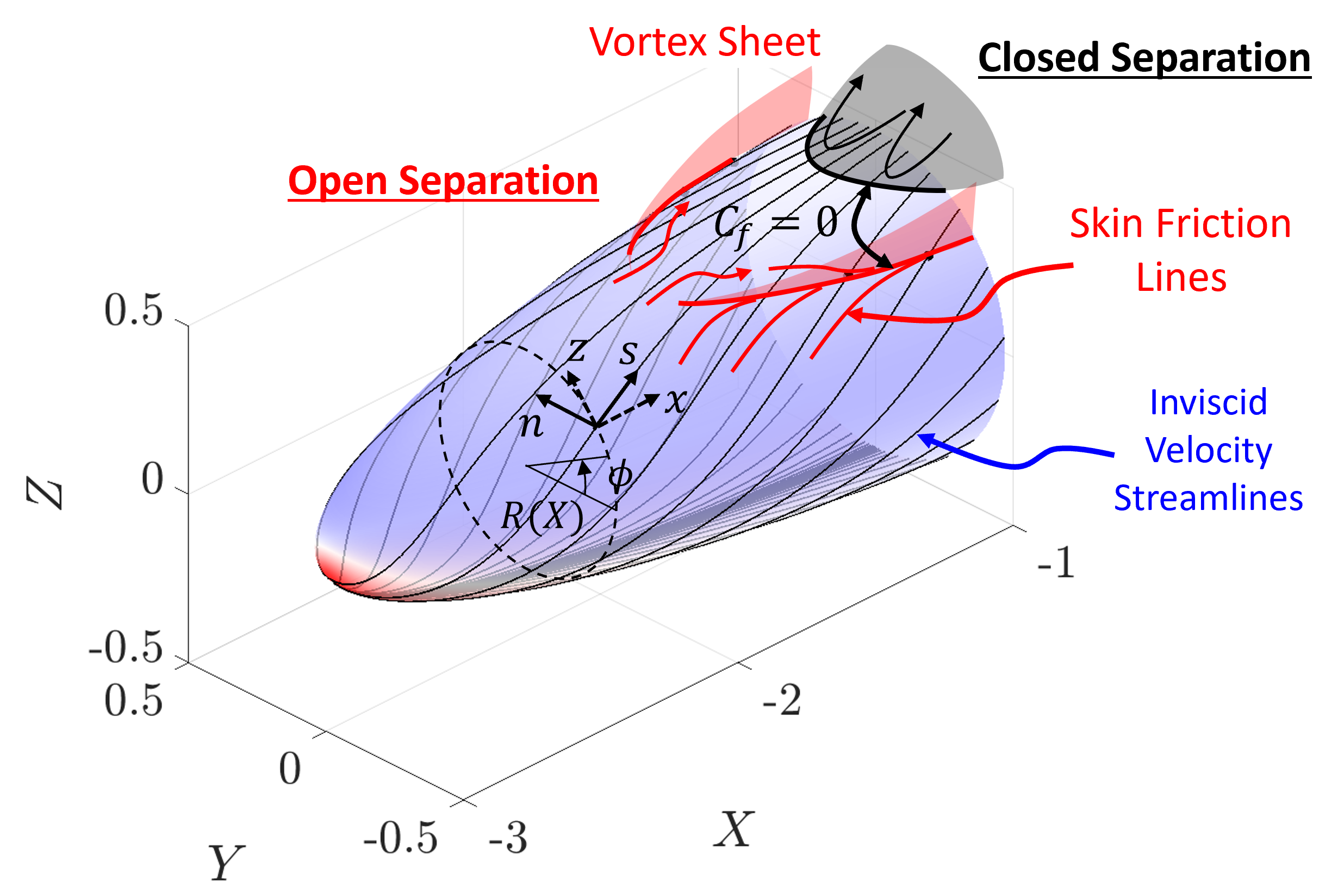
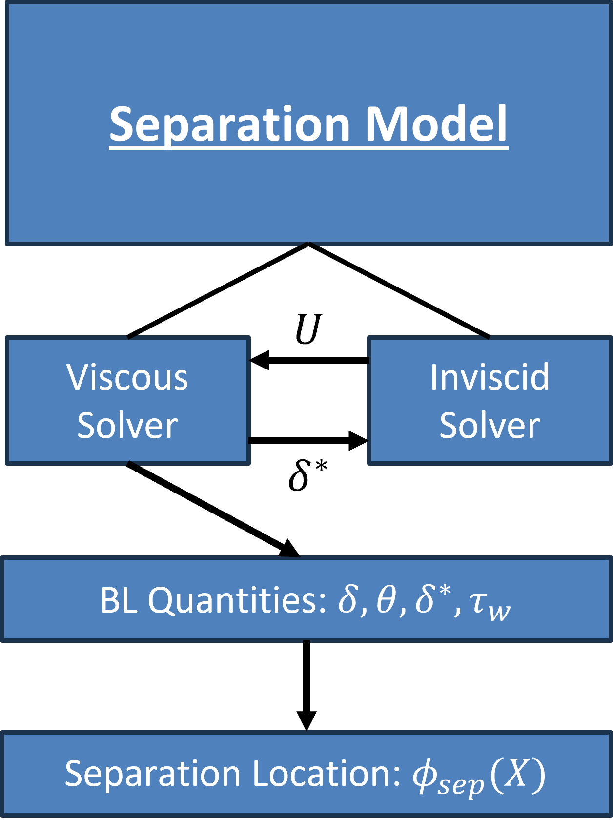
Figure 3 shows a flow chart of the separation model considered in this work. The separation model is based on solving the integral boundary layer equations along streamlines. It has two parts, an inviscid solver based on potential flow theory and a viscous solver based on the boundary layer equations. They are at a minimum one-way coupled where the inviscid solver provides the velocity as a boundary conditon to the viscous solver. Sometimes they are two-way coupled where the displacement thickness, \delta^*, (computed from the viscous solver) is used as a transpiration boundary condition on the inviscid solver. Only one-way coupling is considered in this work.
The viscous solver then outputs boundary layer quantities like the boundary layer thickness, momentum thickness, displacement thickness, and most importantly the wall stress, \tau_w. In the context of this work, separation will be defined as the point where the skin friction or wall stress is zero. This definition is not general and is rather a property of the model itself.
Inviscid Solver
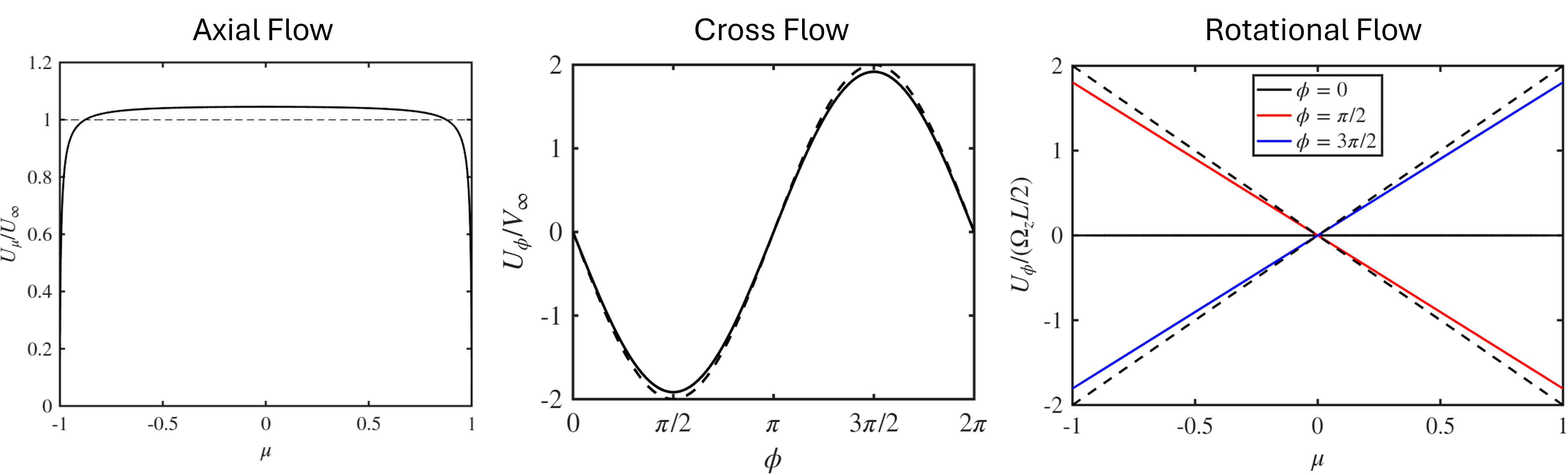
For this preliminary work, the inviscid solution is obtained from analytical solutions given in Lamb (1932). More general methods are possible and will be considered in future work. Figure 4 shows the inviscid velocity for axial flow (flow aligned in X direction), cross flow (flow aligned in Y or Z direction), and rotational flow (flow rotates about the Y or Z axis). The velocity for the axial flow is nearly equal its free stream value because the body is considered slender (length is much larger than diameter). The velocity for the cross flow is very close to inviscid flow over a cylinder, again because the body is slender. And the azimuthal velocity for the rotational flow is similar to the velocity of solid body rotation.
The velocity fields for each of these flows (axial, cross, and rotational) can be superposed to form any type of flow scenario we want. For this work we will primarily be interested in flow at a drift angle (axial + cross) and turning flow (axial + cross + rotational).
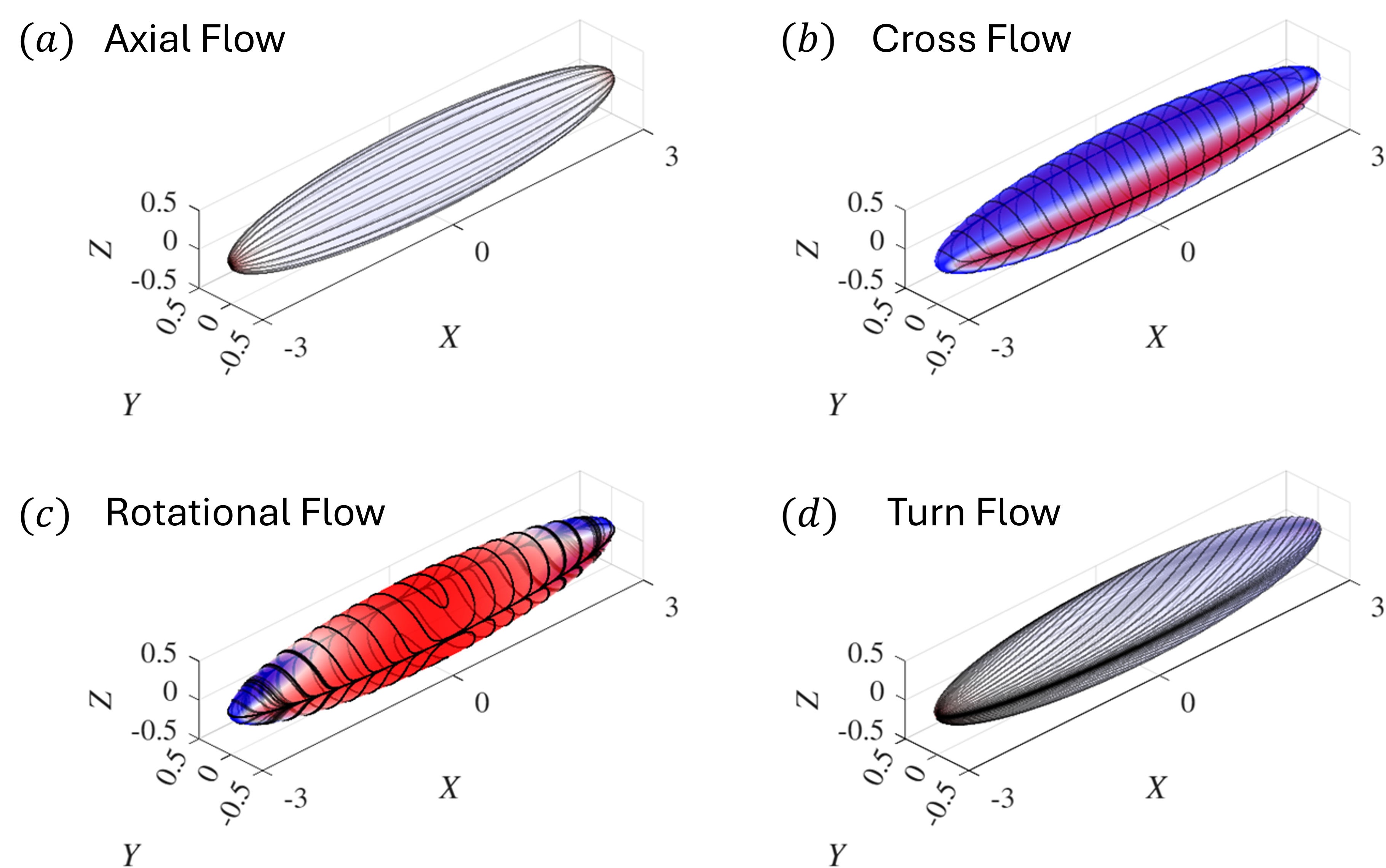
Once the inviscid velocity field is computed we can compute the corresponding streamlines by integrating the velocity vector field. Figure Figure 5 show the resulting streamlines for the axial, cross, rotational, and turn (combination of all three) flows.
Viscous Solver
The viscous solver solves boundary layer equations along the inviscid streamlines with the inviscid velocity used as its outer boundary condition. For now only laminar flow is considered, although transition and turbulence modeling will be added later. The laminar model is based on Thwaites’ method.
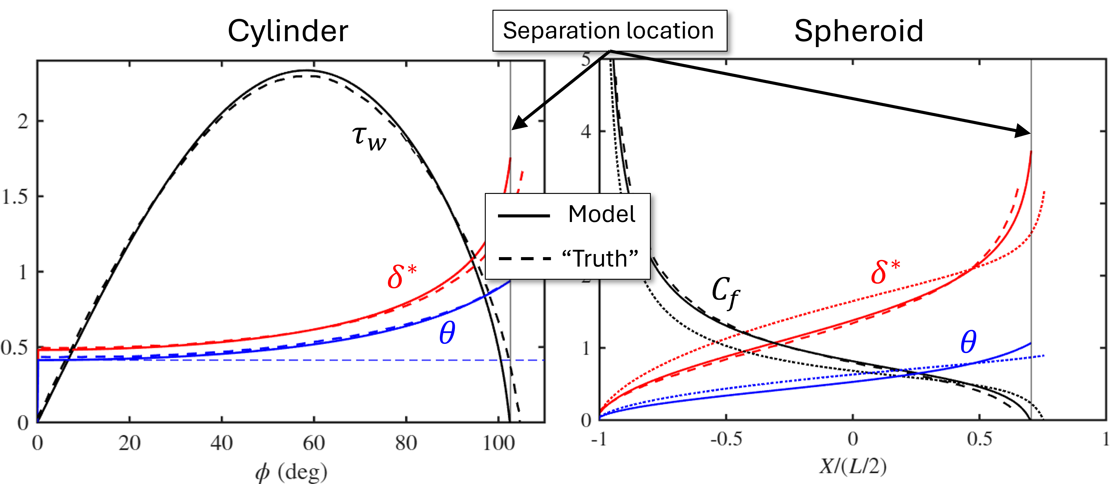
Figure 6 shows the model results (using Thwaites’ method) compared with the “truth” (usually a higher fidelity boundary layer solver) for flow over a cylinder and axial flow over the prolate spheroid. The model and truth agree very well, thus validating the use of Thwaites’ method for these flows. This method is now tested for more general flows.
Results
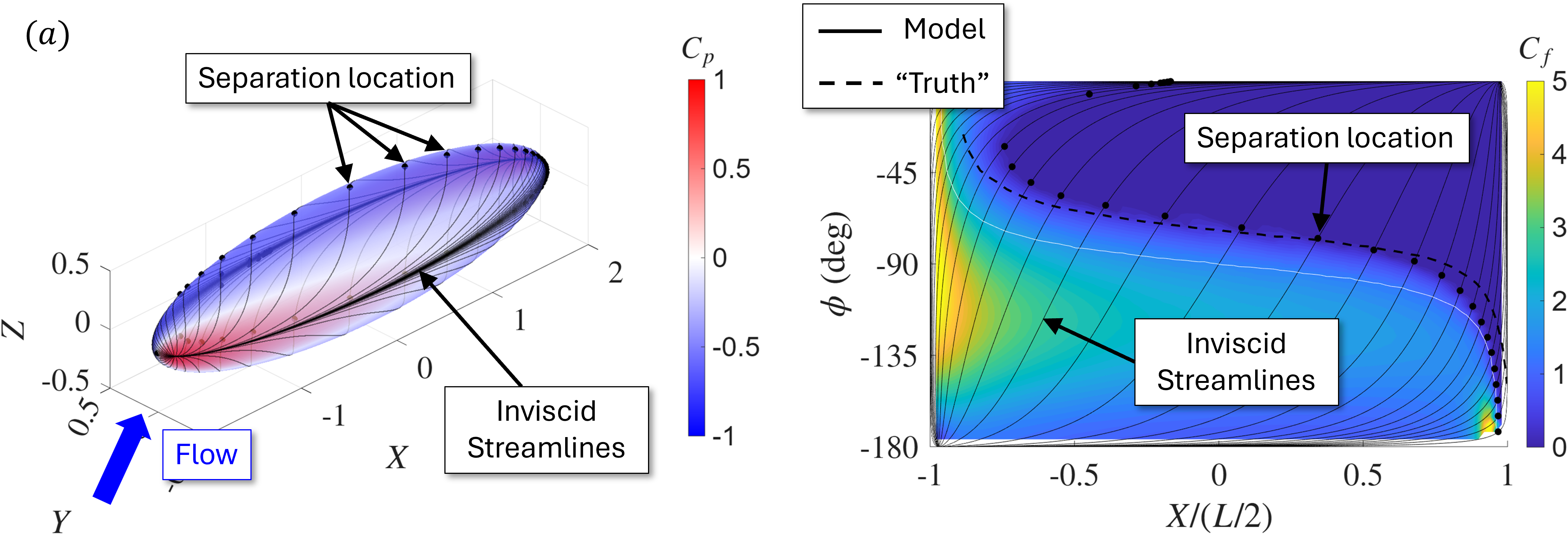
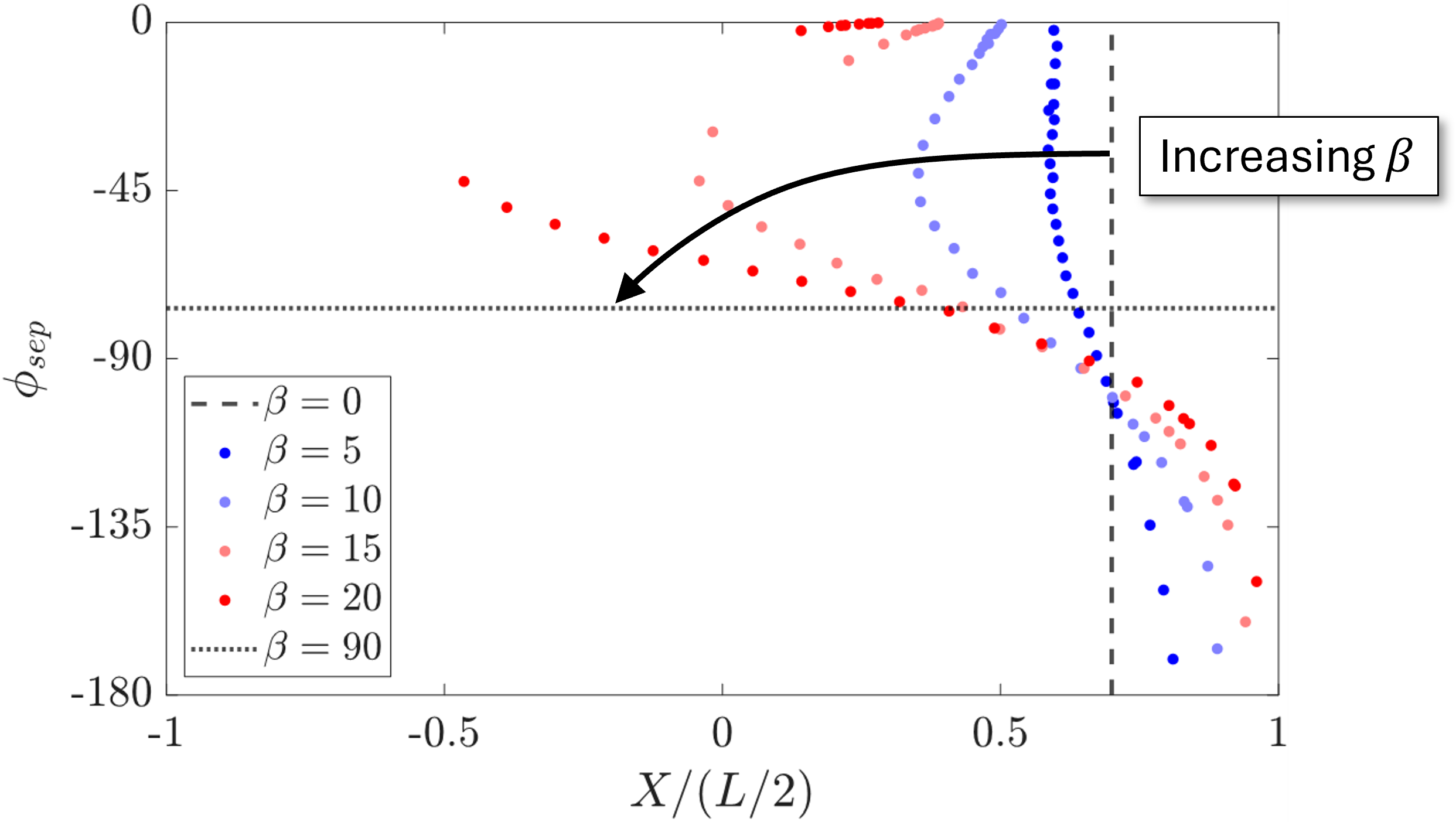
The separation model (inviscid solver + viscous solver) is applied to a prolate spheroid with 30^\circ drift angle and compared with the differential laminar boundary layer solver of Wang (1974) (“Truth”). The model’s separation prediction agrees very well with the truth. The analysis is then extended to multiple drift angles in Figure 8. Here we can qualitative understand the separation trend as the drift angle, \beta, is increased. For \beta = 0^\circ (axial flow) the separation location is constant in X. Then as \beta increases the principle separation location moves further upstream and the curve flattens. For \beta = 90^\circ (cross flow) the separation location is constant.
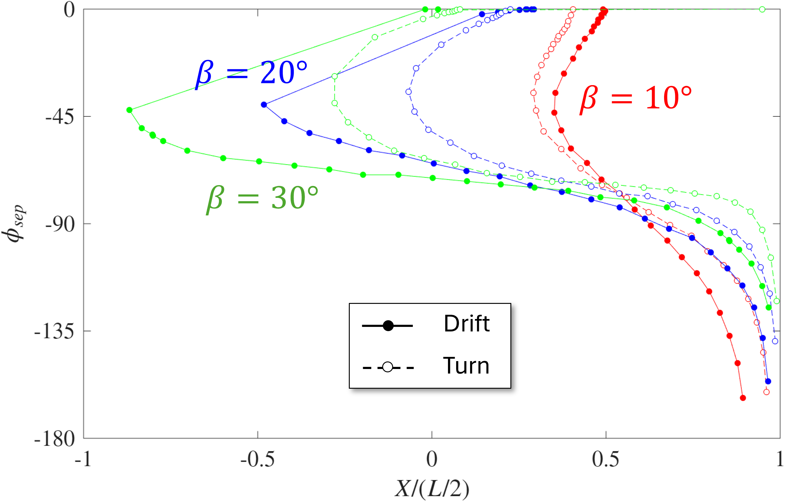
Finally the model is tested for turning flow, to see the effect of rotation on the separation location. Figure 9 compares the separation location for the turn case versus the drift case (no rotation) from before. The effect of rotation on the separation location is complex, with trends being non-monotonic. For high drift angles, turning delays separation whereas for low drift angles, turning causes separation to occur earlier. Further testing needs to be done to validate whether this actually occurs for high fidelity solvers (like RANS, LES, etc.) or if this is just a feature of the model which needs to be improved.